Gradient Descent updates model parameters by calculating the gradient using the entire dataset, providing stable but computationally expensive optimization. Stochastic Gradient Descent approximates this process by updating parameters with each training example, resulting in faster convergence and the ability to escape local minima. Choosing between these methods depends on dataset size, computational resources, and the desired balance between accuracy and training speed.
Table of Comparison
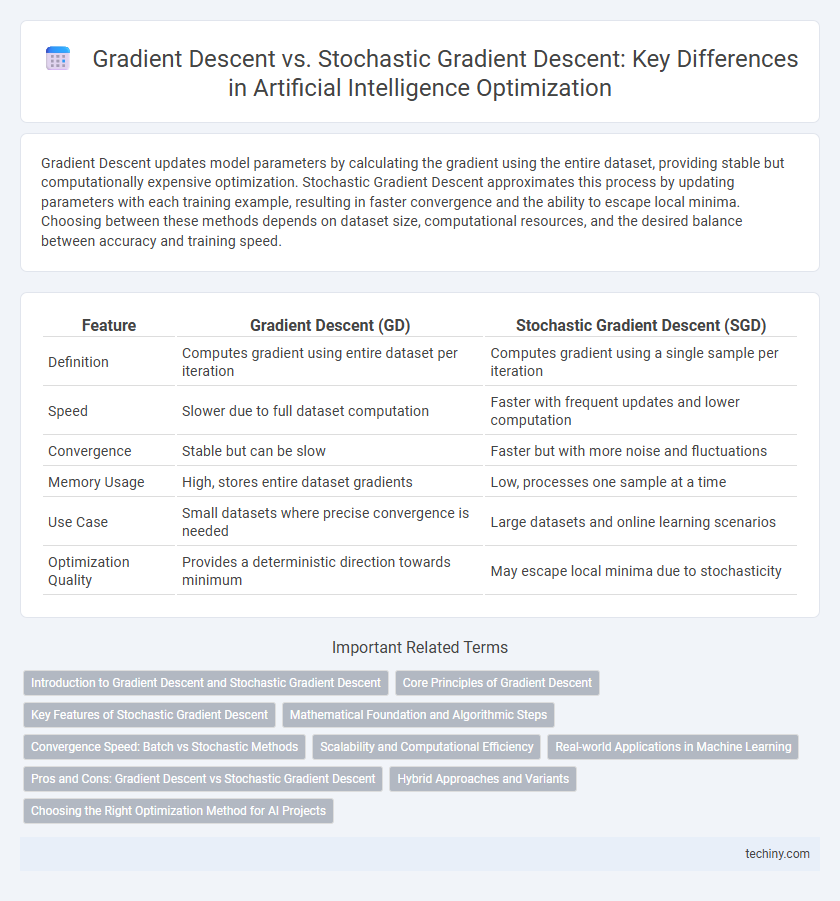
| Feature | Gradient Descent (GD) | Stochastic Gradient Descent (SGD) |
|---|---|---|
| Definition | Computes gradient using entire dataset per iteration | Computes gradient using a single sample per iteration |
| Speed | Slower due to full dataset computation | Faster with frequent updates and lower computation |
| Convergence | Stable but can be slow | Faster but with more noise and fluctuations |
| Memory Usage | High, stores entire dataset gradients | Low, processes one sample at a time |
| Use Case | Small datasets where precise convergence is needed | Large datasets and online learning scenarios |
| Optimization Quality | Provides a deterministic direction towards minimum | May escape local minima due to stochasticity |
Introduction to Gradient Descent and Stochastic Gradient Descent
Gradient Descent is an optimization algorithm used in artificial intelligence to minimize the cost function by iteratively moving towards the steepest descent based on the entire dataset. Stochastic Gradient Descent (SGD) differs by updating model parameters using only one or a few randomly selected data points per iteration, which significantly accelerates convergence especially in large datasets. Both methods are fundamental in training machine learning models, balancing accuracy and computational efficiency.
Core Principles of Gradient Descent
Gradient Descent is an optimization algorithm that minimizes a loss function by iteratively updating model parameters in the direction of the steepest descent, calculated as the negative gradient. This method relies on computing the gradient of the entire dataset's loss function, ensuring stable and smooth convergence towards a global or local minimum. Core principles emphasize the importance of learning rate selection, gradient calculation accuracy, and batch size, which significantly impact the efficiency and effectiveness of the training process in machine learning models.
Key Features of Stochastic Gradient Descent
Stochastic Gradient Descent (SGD) updates model parameters using a single data point or a small batch at each iteration, enabling faster convergence and reduced memory consumption compared to traditional Gradient Descent. Key features of SGD include its ability to escape local minima due to inherent noise in updates, improved scalability for large datasets, and enhanced efficiency in online learning scenarios. This method is particularly advantageous for training deep neural networks where computational resources and dataset size are significant constraints.
Mathematical Foundation and Algorithmic Steps
Gradient Descent optimizes the loss function by computing the gradient across the entire dataset, ensuring precise but computationally intensive updates. Stochastic Gradient Descent (SGD) approximates the gradient using a single randomly selected data point per iteration, significantly speeding up convergence with increased variance in updates. Both algorithms rely on the iterative update rule th = th - eJ(th), where th represents parameters, e the learning rate, and J(th) the gradient, but differ in the granularity of gradient estimation.
Convergence Speed: Batch vs Stochastic Methods
Gradient Descent uses the entire dataset to compute gradients, leading to stable and predictable convergence but often slower updates due to extensive computations. Stochastic Gradient Descent (SGD) computes gradients on individual data points or mini-batches, significantly accelerating convergence speed by enabling more frequent updates. Although SGD introduces higher variance in gradient estimation, its faster iterations often result in quicker approach to optimal solutions in large-scale machine learning tasks.
Scalability and Computational Efficiency
Gradient Descent processes the entire dataset to compute gradients, leading to slower updates but stable convergence, which can hinder scalability with massive datasets. Stochastic Gradient Descent (SGD) updates parameters using individual samples, significantly improving computational efficiency and enabling scalable training for large-scale machine learning models. The trade-off involves SGD's noisier updates but faster iteration cycles, making it preferable for high-dimensional data and real-time applications in artificial intelligence.
Real-world Applications in Machine Learning
Gradient Descent is widely used in training large-scale machine learning models where smooth, deterministic updates optimize loss functions, beneficial for applications like linear regression and neural network training with batch learning. Stochastic Gradient Descent (SGD) excels in real-time model updates and large datasets, improving convergence speed and efficiency in applications such as online recommendation systems, natural language processing, and computer vision. The choice between Gradient Descent and SGD depends on dataset size, computational resources, and the need for model responsiveness in dynamic environments.
Pros and Cons: Gradient Descent vs Stochastic Gradient Descent
Gradient Descent offers stable convergence with precise gradient calculations by processing the entire dataset, making it suitable for small to medium-sized datasets but computationally expensive for large-scale problems. Stochastic Gradient Descent (SGD) updates parameters using single or mini-batches of data points, enabling faster convergence and scalability for large datasets but introducing more noise and less stable convergence. Choosing between Gradient Descent and SGD depends on dataset size, computational resources, and the need for convergence stability versus speed.
Hybrid Approaches and Variants
Hybrid approaches combining Gradient Descent and Stochastic Gradient Descent leverage the stability of batch methods with the efficiency of stochastic optimization, enhancing convergence speed and accuracy in training deep neural networks. Variants such as Mini-Batch Gradient Descent and Adaptive Moment Estimation (Adam) optimize learning rates dynamically while balancing computational costs and noise reduction. These methods have shown significant improvements in handling large-scale datasets and non-convex loss functions in artificial intelligence applications.
Choosing the Right Optimization Method for AI Projects
Choosing the right optimization method in AI projects depends on dataset size and computational resources, with Gradient Descent being effective for smaller datasets due to its stability and convergence accuracy. Stochastic Gradient Descent (SGD) offers faster iterations and better scalability for large-scale data by updating parameters more frequently, which can lead to quicker convergence but higher variance. Hybrid approaches, such as mini-batch gradient descent, balance stability and efficiency, making them suitable for training deep learning models where both speed and precision are critical.
Gradient Descent vs Stochastic Gradient Descent Infographic