L1 regularization promotes sparsity by adding the absolute values of coefficients to the loss function, leading to feature selection and simpler models. L2 regularization adds the squared values of coefficients, encouraging smaller weights and preventing overfitting without eliminating features. Choosing between L1 and L2 depends on the need for feature selection versus model smoothness in artificial intelligence applications.
Table of Comparison
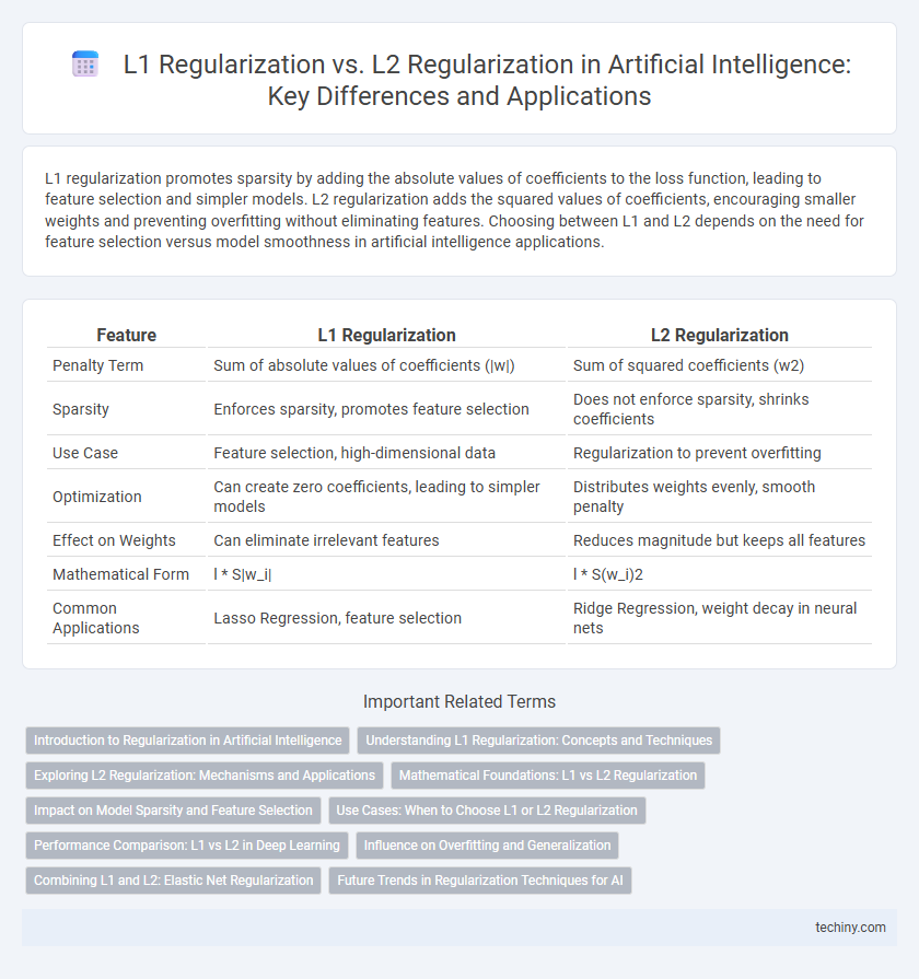
| Feature | L1 Regularization | L2 Regularization |
|---|---|---|
| Penalty Term | Sum of absolute values of coefficients (|w|) | Sum of squared coefficients (w2) |
| Sparsity | Enforces sparsity, promotes feature selection | Does not enforce sparsity, shrinks coefficients |
| Use Case | Feature selection, high-dimensional data | Regularization to prevent overfitting |
| Optimization | Can create zero coefficients, leading to simpler models | Distributes weights evenly, smooth penalty |
| Effect on Weights | Can eliminate irrelevant features | Reduces magnitude but keeps all features |
| Mathematical Form | l * S|w_i| | l * S(w_i)2 |
| Common Applications | Lasso Regression, feature selection | Ridge Regression, weight decay in neural nets |
Introduction to Regularization in Artificial Intelligence
L1 regularization, also known as Lasso, adds the absolute value of coefficients to the loss function, promoting sparsity by driving some weights to zero and enabling feature selection in AI models. L2 regularization, or Ridge, incorporates the squared magnitude of coefficients, reducing model complexity by shrinking weights evenly without eliminating features entirely. Both techniques prevent overfitting in machine learning algorithms by penalizing large parameters, improving generalization and robustness in artificial intelligence systems.
Understanding L1 Regularization: Concepts and Techniques
L1 regularization, also known as Lasso regression, enhances model sparsity by adding a penalty equal to the absolute value of the magnitude of coefficients, effectively promoting feature selection and reducing overfitting. This technique modifies the loss function by incorporating the L1 norm, encouraging many coefficients to become exactly zero, which simplifies the model and improves interpretability. Understanding L1 regularization is essential for tasks involving high-dimensional data where reducing irrelevant features leads to more robust and efficient artificial intelligence algorithms.
Exploring L2 Regularization: Mechanisms and Applications
L2 regularization, also known as Ridge regression, minimizes the sum of squared coefficients to prevent overfitting by penalizing large weights, encouraging model simplicity and stability. Its mechanism involves adding a penalty proportional to the square of the magnitude of coefficients, which effectively distributes error among all parameters and maintains all features in the model. Widely applied in machine learning models such as linear regression, support vector machines, and neural networks, L2 regularization improves generalization performance by reducing model variance without eliminating features entirely.
Mathematical Foundations: L1 vs L2 Regularization
L1 regularization minimizes the sum of absolute values of coefficients, promoting sparsity and feature selection by driving some weights to zero. L2 regularization minimizes the sum of squared coefficients, leading to smaller but non-zero weights, which stabilizes model predictions and reduces overfitting. The optimization for L1 involves the convex but non-smooth absolute value function, while L2 relies on the smooth quadratic function, resulting in different gradient behaviors during training.
Impact on Model Sparsity and Feature Selection
L1 regularization promotes model sparsity by driving many coefficients to exactly zero, effectively performing feature selection and simplifying models in high-dimensional datasets. L2 regularization, by contrast, reduces coefficients uniformly without forcing them to zero, maintaining all features but shrinking their influence and preventing overfitting. The choice between L1 and L2 impacts interpretability and computational efficiency, with L1 favored for explicit feature elimination and L2 for smooth parameter estimation.
Use Cases: When to Choose L1 or L2 Regularization
L1 regularization is preferred in scenarios requiring feature selection or sparsity, making it ideal for high-dimensional datasets where irrelevant features need to be eliminated to improve model interpretability. L2 regularization is more effective in preventing overfitting by shrinking coefficients continuously, making it suitable for models where all input features are believed to contribute to the prediction. When model simplicity and interpretability are priorities, L1 is advantageous; when smooth penalty and stability are desired, especially in regression tasks, L2 proves more beneficial.
Performance Comparison: L1 vs L2 in Deep Learning
L1 regularization promotes sparsity by driving some weights to zero, making it effective for feature selection and producing simpler models, which can enhance interpretability in deep learning. L2 regularization distributes penalties evenly across all weights, encouraging smaller, more evenly distributed values, resulting in smoother models with generally better generalization on unseen data. Performance varies by task and dataset; L1 excels in high-dimensional, sparse settings, while L2 often yields superior accuracy and stability in deep neural networks.
Influence on Overfitting and Generalization
L1 regularization promotes sparsity by driving many model coefficients to zero, effectively performing feature selection which reduces overfitting and can enhance generalization in high-dimensional datasets. L2 regularization penalizes large coefficients by shrinking them towards zero without eliminating features, leading to more stable models that generalize well by distributing weights more evenly. Both techniques mitigate overfitting but differ in their impact on model complexity and interpretability depending on the nature of the data and the learning task.
Combining L1 and L2: Elastic Net Regularization
Elastic Net Regularization effectively combines L1 and L2 regularization by balancing the feature selection strength of L1 with the stability of L2, resulting in improved model generalization and reduced overfitting. This hybrid approach addresses limitations of individual penalties by enabling sparse solutions while maintaining coefficient shrinkage, which is particularly beneficial in high-dimensional datasets with correlated features. Elastic Net's mixing parameter allows fine-tuning the contribution of each regularization term, optimizing performance in various machine learning models such as linear regression and support vector machines.
Future Trends in Regularization Techniques for AI
Future trends in regularization techniques for AI emphasize hybrid approaches that combine L1 and L2 regularization to leverage both sparsity and weight decay benefits. Innovations in adaptive regularization methods are emerging, allowing models to dynamically adjust regularization strength during training based on data complexity and model architecture. Research into novel regularizers inspired by biological neural networks and quantum computing promises to enhance generalization and robustness in next-generation AI systems.
L1 Regularization vs L2 Regularization Infographic