In machine learning, achieving the global optimum ensures the best possible model performance by minimizing the overall loss function, while settling for a local optimum may result in suboptimal predictions due to the algorithm getting trapped in a smaller, less effective solution space. Techniques like stochastic gradient descent with momentum, annealing strategies, and ensemble methods help navigate complex loss landscapes to escape local optima and approach the global minimum. Understanding the distinction between these optima is critical for designing models that generalize well and avoid overfitting or underfitting.
Table of Comparison
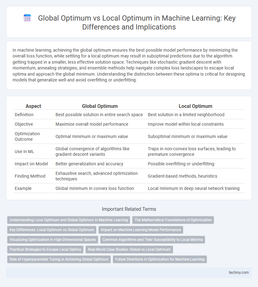
| Aspect | Global Optimum | Local Optimum |
|---|---|---|
| Definition | Best possible solution in entire search space | Best solution in a limited neighborhood |
| Objective | Maximize overall model performance | Improve model within local constraints |
| Optimization Outcome | Optimal minimum or maximum value | Suboptimal minimum or maximum value |
| Use in ML | Global convergence of algorithms like gradient descent variants | Traps in non-convex loss surfaces, leading to premature convergence |
| Impact on Model | Better generalization and accuracy | Possible overfitting or underfitting |
| Finding Method | Exhaustive search, advanced optimization techniques | Gradient-based methods, heuristics |
| Example | Global minimum in convex loss function | Local minimum in deep neural network training |
Understanding Local Optimum and Global Optimum in Machine Learning
Local optimum refers to a solution in machine learning where the algorithm gets stuck in a suboptimal point that is better than its immediate neighbors but not the best overall solution, while the global optimum represents the absolute best solution across the entire search space. Gradient-based optimization methods like stochastic gradient descent often face challenges escaping local optima, leading to suboptimal model performance. Techniques such as simulated annealing, random restarts, and advanced optimizers like Adam help navigate the complex loss landscapes to approach or reach the global optimum.
The Mathematical Foundations of Optimization
The mathematical foundations of optimization in machine learning involve searching for a global optimum, which is the absolute best solution across the entire parameter space, as opposed to a local optimum that represents a suboptimal solution confined within a limited region. Techniques such as gradient descent and its variants navigate complex loss landscapes, often characterized by non-convex functions, where multiple local optima exist and pose challenges to finding the global minimum. Advanced methods like convex optimization, saddle point analysis, and global optimization algorithms leverage mathematical properties to ensure convergence towards the global optimum, enhancing model accuracy and generalization.
Key Differences: Local Optimum vs Global Optimum
Local optimum refers to a solution in machine learning where the model converges to a peak that is better than neighboring solutions but not the best overall, causing suboptimal performance. Global optimum is the absolute best solution across the entire parameter space, ensuring maximum model accuracy or minimum error. Understanding the key difference between local and global optima is critical for designing algorithms that can effectively escape local traps and reach the most accurate predictive models.
Impact on Machine Learning Model Performance
Local optima can significantly limit the performance of machine learning models by trapping optimization algorithms in suboptimal solutions, preventing the discovery of the global optimum that represents the best possible model parameters. Techniques such as stochastic gradient descent, momentum, and adaptive learning rates are employed to navigate complex loss landscapes and escape shallow local optima, thereby enhancing convergence towards the global optimum. Achieving the global optimum improves model generalization, accuracy, and robustness, ultimately leading to more reliable predictions in real-world applications.
Visualizing Optimization in High-Dimensional Spaces
Visualizing optimization in high-dimensional spaces reveals the complexity of navigating toward a global optimum amidst numerous local optima, often characterized by intricate loss landscapes with multiple valleys and peaks. Techniques like t-SNE, PCA, and UMAP help reduce dimensionality, enabling clearer representations of optimization paths and convergence behaviors in neural networks. Understanding these visualizations aids in designing better optimization algorithms that avoid entrapment in suboptimal local minima, improving model performance and generalization.
Common Algorithms and Their Susceptibility to Local Minima
Gradient descent and its variants, including stochastic gradient descent, are common machine learning algorithms highly susceptible to local minima due to their iterative, gradient-based optimization approach. Algorithms like simulated annealing and genetic algorithms mitigate this risk by employing stochastic or population-based search strategies that explore the solution space more broadly. Neural networks, especially deep architectures, frequently encounter local optima, but techniques such as momentum, adaptive learning rates (e.g., Adam optimizer), and batch normalization improve convergence toward the global optimum.
Practical Strategies to Escape Local Optima
Gradient descent with random restarts enhances the chances of finding a global optimum by repeatedly initializing the model at different points in the parameter space. Incorporating techniques like simulated annealing or adding noise to gradients helps the algorithm jump out of local optima and explore more promising regions. Adaptive learning rates and momentum methods further improve convergence speed and robustness against premature trapping in suboptimal solutions.
Real-World Case Studies: Global vs Local Optimum
Real-world case studies in machine learning demonstrate that models often converge to local optima, especially in high-dimensional, non-convex problems like deep neural networks used in image recognition. For instance, Google's AlphaGo utilized reinforcement learning techniques to escape local optima by exploring a broader search space, achieving a global optimum in game strategy. Similarly, autonomous vehicle algorithms rely on global optimum solutions to optimize route planning under dynamic conditions, avoiding suboptimal decisions that local optima might cause.
Role of Hyperparameter Tuning in Achieving Global Optimum
Hyperparameter tuning plays a crucial role in navigating the loss landscape to escape local optima and approach the global optimum in machine learning models. Effective adjustment of learning rate, regularization parameters, and batch size can significantly improve convergence and model performance on complex tasks. Automated techniques like grid search, random search, and Bayesian optimization enhance the discovery of hyperparameter combinations that maximize generalization and minimize overfitting.
Future Directions in Optimization for Machine Learning
Future directions in optimization for machine learning emphasize developing algorithms that better escape local optima to approach global optima, improving model accuracy and robustness. Techniques like meta-learning, adaptive gradient methods, and advanced regularization are being explored to enhance convergence properties in non-convex landscapes. Enhancing interpretability and scalability in complex models remains critical for achieving optimal solutions in large-scale, real-world datasets.
global optimum vs local optimum Infographic